系统工程告诉你如何选择一款最适合的笔记本电脑

背景

由于学习、工作、生活娱乐等需求,小明需要选购一台笔记本电脑,可用于工作(软件开发)、学习(网课)、娱乐(影音、游戏)等。市面上电脑五花八门,小明面临多项选择,如何在经济允许条件下,选择一款满意的笔记本电脑呢?

任务

请运用系统工程的核心——系统分析的思想、流程和方法对于购买电脑这件事进行初步分析,先筛选出若干款产品,再用解释结构模型规范分析影响电脑购买的要素,画出递阶结构模型图,再综合分析进行评价、决策,帮助小明选择自己满意的产品。

一、初步分析理出原始要素

1.1 确定需求

根据题目,小明需要购买笔记本电脑用于学习(网课)、工作(软件开发)和娱乐(影音、游戏),这些需求就是我们的原始要素的基础。

1.2 列出原始要素

  • 性能相关要素
    • $S_1$: 处理器性能(如CPU型号、核心数等)
    • $S_2$: 运存容量(如8GB、16GB等)
    • $S_3$: 存储容量(如256GB SSD、1TB HDD等)
    • $S_4$: 显卡性能(如集成显卡、独立显卡等)
    • $S_5$: 散热性能(如单风扇、双风扇等散热模组)
  • 使用体验相关因素
    • $S_6$: 屏幕尺寸(如13寸、15寸等)
    • $S_7$: 屏幕分辨率(如1080P、4K等)
    • $S_8$: 键盘手感(如键程长短、键帽材质等)
    • $S_9$: 触摸板体验(如是否支持多点触控、灵敏度等)
    • $S_{10}$: 电池续航时间(如4小时、8小时等)
    • $S_{11}$: 重量和便携性(如1.5kg、2kg等)
    • $S_{12}$: 音频效果(如扬声器功率、是否有杜比音效等)
    • $S_{13}$: 接口种类和数量(如USB - A接口数量、是否有HDMI接口等)

二、寻找原始要素的关联关系

2.1 确定关系类型

在这个问题中,关系类型主要考虑“影响”关系,即一个要素的选择会影响另一个要素的选择,而不关系影响的正负反馈类型。

2.2 确定彼此间关系

  • $(S_1, S_2)$: 处理器性能越高,可能需要更大的内存来配合,以避免性能瓶颈。
  • $(S_1, S_3)$: 高性能处理器可能需要更大存储容量来存储大量数据和程序。
  • $(S_1, S_4)$: 高性能处理器可能需要搭配高性能显卡,以满足游戏或图形处理需求。
  • $(S_1, S_5)$: 高性能处理器产生热量多,需要更好的散热性能来维持稳定运行。
  • $(S_2, S_3)$: 大内存通常伴随着对更大存储容量的需求,因为可能需要存储更多的数据和程序。
  • $(S_2, S_4)$: 大内存可以更好地支持高性能显卡处理复杂图形数据。
  • $(S_3, S_4)$: 大存储容量可能需要更好的显卡来处理存储的图形或视频数据。
  • $(S_4, S_5)$: 高性能显卡产生热量多,需要良好的散热系统来保证稳定运行。
  • $(S_5, S_4)$: 散热系统决定了电脑能够安装显卡类型以及显卡型号。
  • $(S_6, S_7)$: 大屏幕通常伴随着高分辨率,以提供更好的视觉体验。
  • $(S_6, S_{11})$: 大屏幕往往导致笔记本电脑重量增加,影响便携性。
  • $(S_7, S_1)$: 高分辨率屏幕需要高性能处理器来处理更多的像素数据。
  • $(S_7, S_9)$: 高分辨率屏幕的触感都比较光滑,会增加触摸感体验。
  • $(S_8, S_{11})$: 如果键盘手感好,可能会增加笔记本的厚度和重量,影响便携性。
  • $(S_9, S_7)$: 多点触控以及较高的灵敏度都会配备较高的屏幕分辨率。
  • $(S_9, S_{11})$: 大触摸板可能会增加笔记本电脑的尺寸和重量。
  • $(S_{10}, S_1)$: 长电池续航时间可能需要低功耗的处理器来实现。
  • $(S_{11}, S_6)$: 较轻的重量设计以及方便携带都会考虑较小的屏幕尺寸。
  • $(S_{12}, S_6)$: 大屏幕可能需要更好的音频效果来匹配观看体验。
  • $(S_{13}, S_{11})$: 接口种类和数量多可能会增加笔记本电脑的厚度和重量。

三、绘制要素间有向关系图

利用 Drawio 软件根据以上确定的要素间关系,绘制出有向关系图,如下图所示:
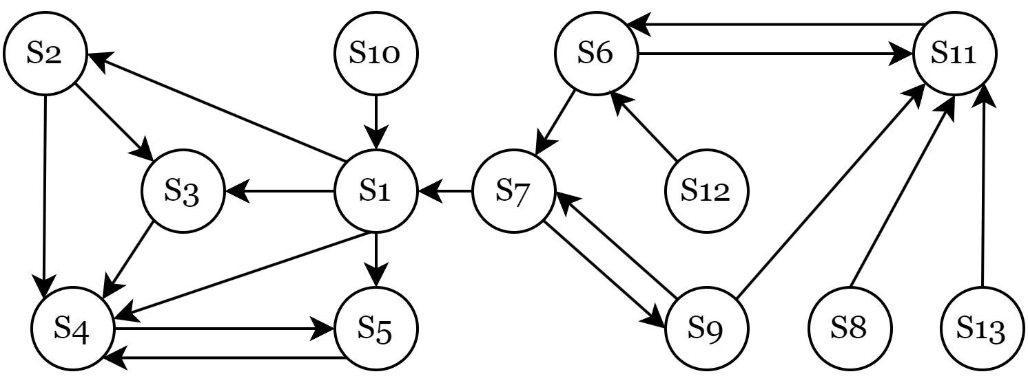
有向关系图

四、系统分析决策类构造

在本文中,我们利用 Python 代码构建了一个名为 DecisionAgent 的类,该类包含了所有系统分析进行决策的处理函数,我们先给出完整的类构造,代码如下:

DecisionAgent Class
1
2
3
4
5
6
7
8
9
10
11
12
13
14
15
16
17
18
19
20
21
22
23
24
25
26
27
28
29
30
31
32
33
34
35
36
37
38
39
40
41
42
43
44
45
46
47
48
49
50
51
52
53
54
55
56
57
58
59
60
61
62
63
64
65
66
67
68
69
70
71
72
73
74
75
76
77
78
79
80
81
82
83
84
85
86
87
88
89
90
91
92
93
94
95
96
97
98
99
100
101
102
103
104
105
106
107
108
109
110
111
112
113
114
115
116
117
118
119
120
121
122
123
124
125
126
127
128
129
130
131
132
133
134
135
136
137
138
139
140
141
142
143
144
145
146
147
148
149
150
151
152
153
154
155
156
157
158
159
160
161
162
163
164
165
166
167
168
169
"""
@author: Zhihao Li
@date: 2024-12-31
@homepage: https://zhihaoli.top/
"""
import numpy as np
import networkx as nx
from collections import defaultdict

class DecisionAgent:
"""
The decision agent class for the decision-making process.
"""
def __init__(self, num_ele):
self.elements = ['S' + str(i) for i in range(1, num_ele + 1)] # list of influential elements
self.adjacency_matrix = np.zeros((num_ele, num_ele)) # adjacency matrix

def set_relations(self, relations_by_ele):
"""
add the relations between the influential elements
"""
relations_pairs = [] # convert to the list of relations pairs
for key in relations_by_ele.keys():
for value in relations_by_ele[key]:
if value != '':
relations_pairs.append([key, value])
print(f">>> relations_pairs:\n{relations_pairs}")
# set the adjacency matrix
for relation in relations_pairs:
self.adjacency_matrix[self.elements.index(relation[0])][self.elements.index(relation[1])] = 1

def get_elements(self):
"""
return the list of influential elements
"""
return self.elements

def get_adjacency_matrix(self):
"""
calculate the adjacency matrix
"""
print(f">>> 原始矩阵 A:\n{self.adjacency_matrix}")
# add self-loop: A = A + I
num = self.adjacency_matrix.shape[0]
self.adjacency_matrix = self.adjacency_matrix + np.eye(num)
print(f">>> 邻接矩阵 I:\n{self.adjacency_matrix}")

def get_reachable_matrix(self):
"""
Get the reachable matrix by the adjacency matrix
"""
# set the reachable matrix
reachable_matrix, step = self.adjacency_matrix.copy(), 1
print(f">>> M{step} = I:\n{reachable_matrix}")
# move to the next step
new_reachable_matrix = np.dot(reachable_matrix, self.adjacency_matrix)
new_reachable_matrix[new_reachable_matrix > 0] = 1
while not np.array_equal(reachable_matrix, new_reachable_matrix):
reachable_matrix = new_reachable_matrix
# move to the next step
new_reachable_matrix = np.dot(reachable_matrix, self.adjacency_matrix)
new_reachable_matrix[new_reachable_matrix > 0] = 1

print(f">>> M{step+1} = M{step} * I:\n{reachable_matrix}")
step += 1

print(f">>> M{step+1} = M{step} * I:\n{reachable_matrix}")
self.reachable_matrix = reachable_matrix
print(f">>> M{step+1} = M{step} ==> R = {step}\n>>> 可达矩阵 M:\n{reachable_matrix}")

def get_reduced_matrix(self):
"""
Get the reduced matrix by the strongly connected components
"""
# construct the drected graph
self.graph = nx.from_numpy_array(self.reachable_matrix, create_using=nx.DiGraph)

# get the strongly connected components
scc = list(nx.strongly_connected_components(self.graph))
# sort the strongly connected components
scc_sorted = [sorted(component) for component in scc]
# sort the strongly connected components by the first element
scc_sorted.sort(key=lambda x: x[0])

# get the representative nodes by the minimum element in each component
representative_nodes = [min(component) for component in scc_sorted]

self.reduced_matrix = self.reachable_matrix[np.ix_(representative_nodes, representative_nodes)]

# display the results
scc_sorted = [[node + 1 for node in component] for component in scc_sorted]
representative_nodes = [node + 1 for node in representative_nodes]

self.headers = ["+".join(f"S{node}" for node in sorted(component)) for component in scc_sorted]
print(">>> 强连通分量 SCC:")
for i, component in enumerate(scc_sorted, start=1):
print(f"\t>>> 连通分量 {i}: {[f'S{node}' for node in sorted(component)]}")
print(f">>> 代表要素:\n{[f'S{node}' for node in sorted(representative_nodes)]}")
reduced_df = pd.DataFrame(self.reduced_matrix.astype(int), index=self.headers, columns=self.headers)
print(f">>> 缩减矩阵:\n{reduced_df}")

print(f">>> 要素表头:\n{self.headers}")


def compute_outdegree(self, matrix, headers):
"""
Compute the out-degree of each node in the matrix
"""
out_degrees = {header: 0 for header in headers}
for i in range(matrix.shape[0]):
for j in range(matrix.shape[1]):
if matrix[i, j] == 1:
out_degrees[headers[i]] += 1

return out_degrees

def compute_indegree(self, matrix, headers):
"""
Compute the in-degree of each node in the matrix
"""
in_degrees = {header: 0 for header in headers}
for i in range(matrix.shape[0]):
for j in range(matrix.shape[1]):
if matrix[i, j] == 1:
in_degrees[headers[j]] += 1

return in_degrees

def layer_summary(self, sorted_elem_outdegree):
"""
Layer summary of the elements by the out-degree
"""
layers = defaultdict(list)
last_outdegree = None
for element, outdegree in sorted_elem_outdegree:
if outdegree != last_outdegree:
last_outdegree = outdegree
layers[outdegree].append(element)

# sort the layers by the out-degree
sorted_layers = sorted(layers.items(), key=lambda x: x[0])
return [layer[1] for layer in sorted_layers]

def get_up_sort_sequence(self):
"""
Get the up sort sequence of the elements
"""
elem_outdegree = self.compute_outdegree(self.reduced_matrix, self.headers)
sorted_elem_outdegree = sorted(elem_outdegree.items(), key=lambda x: x[1])
print(">>> 缩减要素出度排序结果:")
for element, outdegree in sorted_elem_outdegree:
print(f"\t>>> '{element}': {outdegree}")

self.weighted_layers = self.layer_summary(sorted_elem_outdegree)
print(">>> 缩减要素分层汇总结果:")
for i, layer in enumerate(self.weighted_layers, start=1):
print(f"\t>>> 第 {i} 层: {layer}")

def get_backbone_matrix(self):
"""
Get the backbone matrix of the elements
"""
I = np.eye(self.reduced_matrix.shape[0])
self.backbone_matrix = self.reduced_matrix - np.linalg.matrix_power(self.reduced_matrix - I, 2) - I
self.backbone_matrix[self.backbone_matrix < 0] = 0

# Create a DataFrame to display the backbone matrix with headers
backbone_df = pd.DataFrame(self.backbone_matrix.astype(int), index=self.headers, columns=self.headers)
print(f">>> 骨架矩阵 S:\n{backbone_df}")

五、创建要素定义关系

首先需要根据以上定义的要素关系,构造出以要素为分类的语义关系矩阵,然后根据语义关系矩阵导出原始邻接矩阵。

Step 1: 根据要素定义关系创建决策代理以及添加要素关系
1
2
3
4
5
6
7
8
9
10
11
12
13
14
15
16
17
18
19
20
21
22
# 按照要素定义关系
relations_by_ele = {
'S1': ['S2', 'S3', 'S4', 'S5'],
'S2': ['S3', 'S4'],
'S3': ['S4'],
'S4': ['S5'],
'S5': ['S4'],
'S6': ['S7', 'S11'],
'S7': ['S1', 'S9'],
'S8': ['S11'],
'S9': ['S7', 'S11'],
'S10': ['S1'],
'S11': ['S6'],
'S12': ['S6'],
'S13': ['S11']
}
# 根据要素定义关系创建决策代理
agent = DecisionAgent(len(relations_by_ele))
print(f">>> 要素集合:\n{agent.get_elements()}")

# 添加要素关系
agent.set_relations(relations_by_ele)
Step1 Output
1
2
3
4
>>> 要素集合:
['S1', 'S2', 'S3', 'S4', 'S5', 'S6', 'S7', 'S8', 'S9', 'S10', 'S11', 'S12', 'S13']
>>> relations_pairs:
[['S1', 'S2'], ['S1', 'S3'], ['S1', 'S4'], ['S1', 'S5'], ['S2', 'S3'], ['S2', 'S4'], ['S3', 'S4'], ['S4', 'S5'], ['S5', 'S4'], ['S6', 'S7'], ['S6', 'S11'], ['S7', 'S1'], ['S7', 'S9'], ['S8', 'S11'], ['S9', 'S7'], ['S9', 'S11'], ['S10', 'S1'], ['S11', 'S6'], ['S12', 'S6'], ['S13', 'S11']]

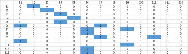
六、根据有向图导出邻接矩阵 $A, I$

邻接矩阵不仅包含了要素之间的关系,还包含了要素的自身关系,因此,邻接矩阵 $I$ 在原始邻接矩阵 $A$ 上还应加入自身的语义关系,即 $I = A + E$,其中 $E$ 为单位矩阵。

Step 2: 根据有向图导出原始矩阵和邻接矩阵
1
2
# 导出原始矩阵和邻接矩阵
agent.get_adjacency_matrix()
Step 2 Output
1
2
3
4
5
6
7
8
9
10
11
12
13
14
15
16
17
18
19
20
21
22
23
24
25
26
27
28
>>> 原始矩阵 A:
[[0. 1. 1. 1. 1. 0. 0. 0. 0. 0. 0. 0. 0.]
[0. 0. 1. 1. 0. 0. 0. 0. 0. 0. 0. 0. 0.]
[0. 0. 0. 1. 0. 0. 0. 0. 0. 0. 0. 0. 0.]
[0. 0. 0. 0. 1. 0. 0. 0. 0. 0. 0. 0. 0.]
[0. 0. 0. 1. 0. 0. 0. 0. 0. 0. 0. 0. 0.]
[0. 0. 0. 0. 0. 0. 1. 0. 0. 0. 1. 0. 0.]
[1. 0. 0. 0. 0. 0. 0. 0. 1. 0. 0. 0. 0.]
[0. 0. 0. 0. 0. 0. 0. 0. 0. 0. 1. 0. 0.]
[0. 0. 0. 0. 0. 0. 1. 0. 0. 0. 1. 0. 0.]
[1. 0. 0. 0. 0. 0. 0. 0. 0. 0. 0. 0. 0.]
[0. 0. 0. 0. 0. 1. 0. 0. 0. 0. 0. 0. 0.]
[0. 0. 0. 0. 0. 1. 0. 0. 0. 0. 0. 0. 0.]
[0. 0. 0. 0. 0. 0. 0. 0. 0. 0. 1. 0. 0.]]
>>> 邻接矩阵 I:
[[1. 1. 1. 1. 1. 0. 0. 0. 0. 0. 0. 0. 0.]
[0. 1. 1. 1. 0. 0. 0. 0. 0. 0. 0. 0. 0.]
[0. 0. 1. 1. 0. 0. 0. 0. 0. 0. 0. 0. 0.]
[0. 0. 0. 1. 1. 0. 0. 0. 0. 0. 0. 0. 0.]
[0. 0. 0. 1. 1. 0. 0. 0. 0. 0. 0. 0. 0.]
[0. 0. 0. 0. 0. 1. 1. 0. 0. 0. 1. 0. 0.]
[1. 0. 0. 0. 0. 0. 1. 0. 1. 0. 0. 0. 0.]
[0. 0. 0. 0. 0. 0. 0. 1. 0. 0. 1. 0. 0.]
[0. 0. 0. 0. 0. 0. 1. 0. 1. 0. 1. 0. 0.]
[1. 0. 0. 0. 0. 0. 0. 0. 0. 1. 0. 0. 0.]
[0. 0. 0. 0. 0. 1. 0. 0. 0. 0. 1. 0. 0.]
[0. 0. 0. 0. 0. 1. 0. 0. 0. 0. 0. 1. 0.]
[0. 0. 0. 0. 0. 0. 0. 0. 0. 0. 1. 0. 1.]]

七、根据邻接矩阵导出可达矩阵 $M$

可达矩阵 $M$ 是邻接矩阵 $I$ 的幂级数,其计算公式为 $M = I^k$,其中 $k$ 为最高可达次数。由于 $I$ 为对称矩阵,因此 $M$ 也是对称矩阵。

Step 3: 根据邻接矩阵导出可达矩阵
1
2
# 导出可达矩阵
agent.get_reachable_matrix()
Step 3 Output
1
2
3
4
5
6
7
8
9
10
11
12
13
14
15
16
17
18
19
20
21
22
23
24
25
26
27
28
29
30
31
32
33
34
35
36
37
38
39
40
41
42
43
44
45
46
47
48
49
50
51
52
53
54
55
56
57
58
59
60
61
62
63
64
65
66
67
68
69
70
71
72
73
74
75
76
77
78
79
80
81
82
83
84
85
86
87
88
89
90
91
92
93
94
95
96
97
98
99
>>> M1 = I:
[[1. 1. 1. 1. 1. 0. 0. 0. 0. 0. 0. 0. 0.]
[0. 1. 1. 1. 0. 0. 0. 0. 0. 0. 0. 0. 0.]
[0. 0. 1. 1. 0. 0. 0. 0. 0. 0. 0. 0. 0.]
[0. 0. 0. 1. 1. 0. 0. 0. 0. 0. 0. 0. 0.]
[0. 0. 0. 1. 1. 0. 0. 0. 0. 0. 0. 0. 0.]
[0. 0. 0. 0. 0. 1. 1. 0. 0. 0. 1. 0. 0.]
[1. 0. 0. 0. 0. 0. 1. 0. 1. 0. 0. 0. 0.]
[0. 0. 0. 0. 0. 0. 0. 1. 0. 0. 1. 0. 0.]
[0. 0. 0. 0. 0. 0. 1. 0. 1. 0. 1. 0. 0.]
[1. 0. 0. 0. 0. 0. 0. 0. 0. 1. 0. 0. 0.]
[0. 0. 0. 0. 0. 1. 0. 0. 0. 0. 1. 0. 0.]
[0. 0. 0. 0. 0. 1. 0. 0. 0. 0. 0. 1. 0.]
[0. 0. 0. 0. 0. 0. 0. 0. 0. 0. 1. 0. 1.]]
>>> M2 = M1 * I:
[[1. 1. 1. 1. 1. 0. 0. 0. 0. 0. 0. 0. 0.]
[0. 1. 1. 1. 1. 0. 0. 0. 0. 0. 0. 0. 0.]
[0. 0. 1. 1. 1. 0. 0. 0. 0. 0. 0. 0. 0.]
[0. 0. 0. 1. 1. 0. 0. 0. 0. 0. 0. 0. 0.]
[0. 0. 0. 1. 1. 0. 0. 0. 0. 0. 0. 0. 0.]
[1. 0. 0. 0. 0. 1. 1. 0. 1. 0. 1. 0. 0.]
[1. 1. 1. 1. 1. 0. 1. 0. 1. 0. 1. 0. 0.]
[0. 0. 0. 0. 0. 1. 0. 1. 0. 0. 1. 0. 0.]
[1. 0. 0. 0. 0. 1. 1. 0. 1. 0. 1. 0. 0.]
[1. 1. 1. 1. 1. 0. 0. 0. 0. 1. 0. 0. 0.]
[0. 0. 0. 0. 0. 1. 1. 0. 0. 0. 1. 0. 0.]
[0. 0. 0. 0. 0. 1. 1. 0. 0. 0. 1. 1. 0.]
[0. 0. 0. 0. 0. 1. 0. 0. 0. 0. 1. 0. 1.]]
>>> M3 = M2 * I:
[[1. 1. 1. 1. 1. 0. 0. 0. 0. 0. 0. 0. 0.]
[0. 1. 1. 1. 1. 0. 0. 0. 0. 0. 0. 0. 0.]
[0. 0. 1. 1. 1. 0. 0. 0. 0. 0. 0. 0. 0.]
[0. 0. 0. 1. 1. 0. 0. 0. 0. 0. 0. 0. 0.]
[0. 0. 0. 1. 1. 0. 0. 0. 0. 0. 0. 0. 0.]
[1. 1. 1. 1. 1. 1. 1. 0. 1. 0. 1. 0. 0.]
[1. 1. 1. 1. 1. 1. 1. 0. 1. 0. 1. 0. 0.]
[0. 0. 0. 0. 0. 1. 1. 1. 0. 0. 1. 0. 0.]
[1. 1. 1. 1. 1. 1. 1. 0. 1. 0. 1. 0. 0.]
[1. 1. 1. 1. 1. 0. 0. 0. 0. 1. 0. 0. 0.]
[1. 0. 0. 0. 0. 1. 1. 0. 1. 0. 1. 0. 0.]
[1. 0. 0. 0. 0. 1. 1. 0. 1. 0. 1. 1. 0.]
[0. 0. 0. 0. 0. 1. 1. 0. 0. 0. 1. 0. 1.]]
>>> M4 = M3 * I:
[[1. 1. 1. 1. 1. 0. 0. 0. 0. 0. 0. 0. 0.]
[0. 1. 1. 1. 1. 0. 0. 0. 0. 0. 0. 0. 0.]
[0. 0. 1. 1. 1. 0. 0. 0. 0. 0. 0. 0. 0.]
[0. 0. 0. 1. 1. 0. 0. 0. 0. 0. 0. 0. 0.]
[0. 0. 0. 1. 1. 0. 0. 0. 0. 0. 0. 0. 0.]
[1. 1. 1. 1. 1. 1. 1. 0. 1. 0. 1. 0. 0.]
[1. 1. 1. 1. 1. 1. 1. 0. 1. 0. 1. 0. 0.]
[1. 0. 0. 0. 0. 1. 1. 1. 1. 0. 1. 0. 0.]
[1. 1. 1. 1. 1. 1. 1. 0. 1. 0. 1. 0. 0.]
[1. 1. 1. 1. 1. 0. 0. 0. 0. 1. 0. 0. 0.]
[1. 1. 1. 1. 1. 1. 1. 0. 1. 0. 1. 0. 0.]
[1. 1. 1. 1. 1. 1. 1. 0. 1. 0. 1. 1. 0.]
[1. 0. 0. 0. 0. 1. 1. 0. 1. 0. 1. 0. 1.]]
>>> M5 = M4 * I:
[[1. 1. 1. 1. 1. 0. 0. 0. 0. 0. 0. 0. 0.]
[0. 1. 1. 1. 1. 0. 0. 0. 0. 0. 0. 0. 0.]
[0. 0. 1. 1. 1. 0. 0. 0. 0. 0. 0. 0. 0.]
[0. 0. 0. 1. 1. 0. 0. 0. 0. 0. 0. 0. 0.]
[0. 0. 0. 1. 1. 0. 0. 0. 0. 0. 0. 0. 0.]
[1. 1. 1. 1. 1. 1. 1. 0. 1. 0. 1. 0. 0.]
[1. 1. 1. 1. 1. 1. 1. 0. 1. 0. 1. 0. 0.]
[1. 1. 1. 1. 1. 1. 1. 1. 1. 0. 1. 0. 0.]
[1. 1. 1. 1. 1. 1. 1. 0. 1. 0. 1. 0. 0.]
[1. 1. 1. 1. 1. 0. 0. 0. 0. 1. 0. 0. 0.]
[1. 1. 1. 1. 1. 1. 1. 0. 1. 0. 1. 0. 0.]
[1. 1. 1. 1. 1. 1. 1. 0. 1. 0. 1. 1. 0.]
[1. 1. 1. 1. 1. 1. 1. 0. 1. 0. 1. 0. 1.]]
>>> M6 = M5 * I:
[[1. 1. 1. 1. 1. 0. 0. 0. 0. 0. 0. 0. 0.]
[0. 1. 1. 1. 1. 0. 0. 0. 0. 0. 0. 0. 0.]
[0. 0. 1. 1. 1. 0. 0. 0. 0. 0. 0. 0. 0.]
[0. 0. 0. 1. 1. 0. 0. 0. 0. 0. 0. 0. 0.]
[0. 0. 0. 1. 1. 0. 0. 0. 0. 0. 0. 0. 0.]
[1. 1. 1. 1. 1. 1. 1. 0. 1. 0. 1. 0. 0.]
[1. 1. 1. 1. 1. 1. 1. 0. 1. 0. 1. 0. 0.]
[1. 1. 1. 1. 1. 1. 1. 1. 1. 0. 1. 0. 0.]
[1. 1. 1. 1. 1. 1. 1. 0. 1. 0. 1. 0. 0.]
[1. 1. 1. 1. 1. 0. 0. 0. 0. 1. 0. 0. 0.]
[1. 1. 1. 1. 1. 1. 1. 0. 1. 0. 1. 0. 0.]
[1. 1. 1. 1. 1. 1. 1. 0. 1. 0. 1. 1. 0.]
[1. 1. 1. 1. 1. 1. 1. 0. 1. 0. 1. 0. 1.]]
>>> M6 = M5 ==> R = 5
>>> 可达矩阵 M:
[[1. 1. 1. 1. 1. 0. 0. 0. 0. 0. 0. 0. 0.]
[0. 1. 1. 1. 1. 0. 0. 0. 0. 0. 0. 0. 0.]
[0. 0. 1. 1. 1. 0. 0. 0. 0. 0. 0. 0. 0.]
[0. 0. 0. 1. 1. 0. 0. 0. 0. 0. 0. 0. 0.]
[0. 0. 0. 1. 1. 0. 0. 0. 0. 0. 0. 0. 0.]
[1. 1. 1. 1. 1. 1. 1. 0. 1. 0. 1. 0. 0.]
[1. 1. 1. 1. 1. 1. 1. 0. 1. 0. 1. 0. 0.]
[1. 1. 1. 1. 1. 1. 1. 1. 1. 0. 1. 0. 0.]
[1. 1. 1. 1. 1. 1. 1. 0. 1. 0. 1. 0. 0.]
[1. 1. 1. 1. 1. 0. 0. 0. 0. 1. 0. 0. 0.]
[1. 1. 1. 1. 1. 1. 1. 0. 1. 0. 1. 0. 0.]
[1. 1. 1. 1. 1. 1. 1. 0. 1. 0. 1. 1. 0.]
[1. 1. 1. 1. 1. 1. 1. 0. 1. 0. 1. 0. 1.]]

八、根据强连通分量计算缩减矩阵

首先需要寻找语义关系图中的强连通分量,根据强连通分量确定可以缩减为一组的各个影响因素。将具有强连接关系的一组要素看作一个要素,保留其中某个代表要素,删除掉其余要素在 $M$ 中的行和列。

Step 4: 根据强连通分量计算缩减矩阵
1
2
# 计算缩减矩阵
agent.get_reduced_matrix()
Step 4 Output
1
2
3
4
5
6
7
8
9
10
11
12
13
14
15
16
17
18
19
20
21
22
23
24
25
>>> 强连通分量 SCC:
>>> 连通分量 1: ['S1']
>>> 连通分量 2: ['S2']
>>> 连通分量 3: ['S3']
>>> 连通分量 4: ['S4', 'S5']
>>> 连通分量 5: ['S6', 'S7', 'S9', 'S11']
>>> 连通分量 6: ['S8']
>>> 连通分量 7: ['S10']
>>> 连通分量 8: ['S12']
>>> 连通分量 9: ['S13']
>>> 代表要素:
['S1', 'S2', 'S3', 'S4', 'S6', 'S8', 'S10', 'S12', 'S13']
>>> 缩减矩阵:
S1 S2 S3 S4+S5 S6+S7+S9+S11 S8 S10 S12 S13
S1 1 1 1 1 0 0 0 0 0
S2 0 1 1 1 0 0 0 0 0
S3 0 0 1 1 0 0 0 0 0
S4+S5 0 0 0 1 0 0 0 0 0
S6+S7+S9+S11 1 1 1 1 1 0 0 0 0
S8 1 1 1 1 1 1 0 0 0
S10 1 1 1 1 0 0 1 0 0
S12 1 1 1 1 1 0 0 1 0
S13 1 1 1 1 1 0 0 0 1
>>> 要素表头:
['S1', 'S2', 'S3', 'S4+S5', 'S6+S7+S9+S11', 'S8', 'S10', 'S12', 'S13']

九、对缩减后的各要素组进行排序

排序的原则是要素的出度,按照升序的原则对各要素组排序,最高级的要素是系统的终止集要素,是只受其他要素影响(到达)的要素所构成的集合。在有向图中表示只有箭头流入,而无箭线流出,是系统的输出要素。

根据以上原则,我们对缩减后的要素组进行排序,得到排序后的要素组。

Step 5: 按照结果升序排序要素组
1
2
# 得到加权排序的要素分层汇总结果
agent.get_up_sort_sequence()
Step 5 Output
1
2
3
4
5
6
7
8
9
10
11
12
13
14
15
16
17
18
>>> 排序后的要素组:
>>> 缩减要素出度排序结果:
>>> 'S4+S5': 1
>>> 'S3': 2
>>> 'S2': 3
>>> 'S1': 4
>>> 'S6+S7+S9+S11': 5
>>> 'S10': 5
>>> 'S8': 6
>>> 'S12': 6
>>> 'S13': 6
>>> 缩减要素分层汇总结果:
>>> 第 1 层: ['S4+S5']
>>> 第 2 层: ['S3']
>>> 第 3 层: ['S2']
>>> 第 4 层: ['S1']
>>> 第 5 层: ['S6+S7+S9+S11', 'S10']
>>> 第 6 层: ['S8', 'S12', 'S13']

最后,根据出度排序进行缩减矩阵行列变换:
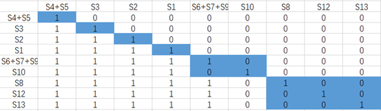
缩减矩阵变换

十、计算骨架矩阵并构建梯阶模型

由缩减后的可达矩阵 $M’$ 计算得到骨架矩阵,即 $S = M’ - (M’-I)^2 -I$,其中 $I$ 为单位矩阵。

Step 6: 计算骨架矩阵
1
2
# 得到骨架矩阵
agent.get_backbone_matrix()
Step 6 Output
1
2
3
4
5
6
7
8
9
10
11
>>> 骨架矩阵 S:
S1 S2 S3 S4+S5 S6+S7+S9+S11 S8 S10 S12 S13
S1 0 1 0 0 0 0 0 0 0
S2 0 0 1 0 0 0 0 0 0
S3 0 0 0 1 0 0 0 0 0
S4+S5 0 0 0 0 0 0 0 0 0
S6+S7+S9+S11 1 0 0 0 0 0 0 0 0
S8 0 0 0 0 1 0 0 0 0
S10 1 0 0 0 0 0 0 0 0
S12 0 0 0 0 1 0 0 0 0
S13 0 0 0 0 1 0 0 0 0

结合要素分层结果以及骨架矩阵,我们可以构建出梯阶模型,即:

  1. 从上到下逐级排列系统构成要素;
  2. 同级加入被删除的与某要素有强连接关系的要素及表征他们相互关系的有向弧;
  3. 用级间有向弧连接成有向图。
梯阶结构模型

进一步地,以菊花链表示回路,根据梯阶模型将其转换为一般性骨架矩阵 $S’$。

一般性骨架矩阵

十一、决策方案

候选产品

  1. 机械革命无界14X(4000 元左右)
    • 处理器:R7-8845HS,显卡:Radeon 780M
    • 屏幕:14英寸,2.8K,120Hz
    • 电池:80Wh,重量:1.45kg
  2. 惠普战66七代锐龙版(4000 元左右)
    • 处理器:R7 7735U,显卡:集显
    • 屏幕:14英寸,2.5K,120Hz
    • 电池:56Wh,重量:1.4kg
  3. 荣耀MagicBook X14Pro(3500 元左右)
    • 处理器:R7-7840HS,显卡:核显
    • 屏幕:14英寸,1080P,60Hz
    • 电池:60Wh,重量:1.4kg
  4. 宏碁非凡Go Pro(4000 元左右)
    • 处理器:i5-13500H,显卡:核显
    • 屏幕:14英寸,2.8K,120Hz
    • 电池:60Wh,重量:1.49kg
  5. Thinkbook14 2023(4000 元左右)
    • 处理器:i5-13500H,显卡:核显
    • 屏幕:14英寸,2.2K,高色域
    • 电池:60Wh,重量:1.42kg
  6. 联想小新Pro14锐龙版(5000 元左右)
    • 处理器:R7-8745H,显卡:核显
    • 屏幕:14英寸,2.8K,120Hz
    • 电池:84Wh,重量:1.46kg
  7. Redmibook Pro14(5000 元左右)
    • 处理器:Ultra5-125H,显卡:核显
    • 屏幕:14英寸,2.8K,120Hz
    • 电池:80Wh,重量:1.46kg
  8. 联想拯救者R7000(7000 元左右)
    • 处理器:i7-13650HX,显卡:RTX4060
    • 屏幕:15.6英寸,1080P,144Hz
    • 电池:60Wh,重量:2.35kg
  9. 惠普暗影精灵乐享版(7000 元左右)
    • 处理器:i7-14650HX,显卡:RTX4060
    • 屏幕:16.1英寸,2.5K,240Hz
    • 电池:83Wh,重量:2.4kg

具体分析

层次分析

  1. 第一层:S4(显卡性能),S5(散热性能)是小明考虑的主要因素。

    显卡主要是负责笔记本电脑图像、图形输出任务,分为核显与独显,核显搭载在轻薄本上,图形性能一般,适合办公、影音娱乐,玩玩网游等使用需求,比较省电。独显就是独立的显卡,图形性能强,一般搭载在全能本、游戏本上,适合玩大型3A游戏、专业创作设计、三维建模、视频渲染等需求。同时笔记本电脑的散热性能对于性能和舒适度都非常重要。散热系统的好坏会影响CPU和GPU的性能。

  2. 第二层:S3(存储容量)是小明需要考虑的重要因素。

    存储容量是衡量电脑能存储多少信息(如文档、图片、视频和安装的程序)的关键指标。一个高存储容量的电脑能够存储更多的文件和应用程序,从而提高用户的使用便利性。

  3. 第三层:S2(内存容量)是小明需要考虑的重要因素。

    内存容量大小影响运行速度快慢。笔记本电脑内存容量标配16G,对于办公、玩网游、业余创作设计等来说够用了,如果有编程、写代码、多开虚拟机,跑仿真、多开大量软件等需求,建议内存容量选择32G。

  4. 第四层:S1(处理器性能)是小明需要考虑的重要因素。

    处理器相当于笔记本电脑的大脑,是最核心的硬件,用来处理和计算各种复杂指令,运行程序等,处理器性能决定了电脑处理任务的速度。

  5. 第五层:S10(电池续航时间),S6(屏幕尺寸),S7(屏幕分辨率),S9(触摸板体验),S11(重量和便携性)是小明需要考虑的较重要因素。

    这些因素共同影响着笔记本的使用体验,电池续航时间过短意味着笔记本需要经常充电,无法长时间在外办公学习,屏幕尺寸和屏幕分辨率影响使用者看视频、网课的体验,触摸板灵敏度影响使用者的使用体验,重量影响笔记本的可携带性。

  6. 第六层:S8(键盘手感),S12(音频效果),S13(接口种类和数量)是小明需要考虑的次要因素。

    在必要时刻可以较低需求,满足基本需要即可。

具体选择

考虑到小明的具体需求:学习(网课)、工作(软件开发)和娱乐(影音、游戏)和上述因素,我们做出具体选择:

  1. 若小明预算充足(7000 元左右),可以选择惠普暗影精灵乐享版,搭载最新Intel酷睿14代处理器,i7-14650HX性能释放激进,多核性能表现较好,高负载情况下核心温度较低。屏幕显示素质较好,支持2.5K高分辨率,240Hz刷新率。拓展性好,接口丰富,可以满足小明的各种需求。联想拯救者R7000虽然各方面性能也不错,但是是塑料机身,平时携带外出损坏可能较惠普更大。
  2. 若小明预算在 4000-5000 元之间,可以选择惠普战66七代锐龙版,联想小新Pro14锐龙版。惠普战66七代锐龙版采用AMD锐龙7 7735U处理器,可满足办公之类需求。全金属机身机,身质感好,打字手感好。屏幕支持2.5K高分辨率,120Hz刷新率,500nit高亮度,同价位非常少见。拓展性好,接口种类丰富,数量多。而联想小新Pro14锐龙版有24G大内存,内存容量非常充足,核显性能超过独显MX570,可以低画质60帧左右大型游戏。处理器是最新的AMD锐龙8000系,功耗最高可达63W。搭载了84Wh大电池,续航能力相对较好。两种笔记本都可以满足小明的具体需求。机械革命无界14X散热性能较差且售后一般,荣耀MagicBook X14Pro,宏碁非凡Go Pro接口较少,不够全面,Thinkbook14 2023内存容量较低,会限制用户在使用时有效地分配资源,Redmibook Pro14键盘手感可能不好,影响小明进行软件开发。

参考

曾浩. 2024年秋, 工程概论(IV), 西安电子科技大学.

https://mooc1.chaoxing.com/mooc-ans/course/244962689.html

系统工程告诉你如何选择一款最适合的笔记本电脑

https://lzhms.github.io/blog/DecisionAgent/

Author

Zhihao Li

Posted on

2024-12-31

Updated on

2025-03-09

Licensed under


Comments